当我们要解决一个分类问题,尤其是一个二分类问题时,如果我们用线性回归去解决就会面临这样一个问题:样本量变大后,准确率会下降。这时为了更好地解决这种分类问题,我们就需要采用逻辑回归的方法了。现在有两个逻辑回归的实战案例:考试通过预测、芯片检测通过预测。同样本次练习也是基于sk-learn库, 通过逻辑回归实现二分类。
<!-- more --> <!--more-->
一、考试通过预测
首先看第一个目标:基于数据集建立逻辑回归模型,并预测给定两门分数的情况下,预测第三门分数是否能通过;建立二阶边界,提高模型的准确率。
下面的内容基本就是Jupyter NoteBook的内容了:
-
1.基于testdata.csv数据,建立逻辑回归模型,评估模型的表现。
-
2.预测Exam1 = 75,Exam2 = 60 时,该同学能否通过 Exam3。
-
3.建立二阶边界函数,重复任务1,2步骤。
#load from csv
import pandas as pd
import numpy as np

data = pd.read_csv('examdata.csv')
data.head()
<table border="1" class="dataframe"> <thead> <tr style="text-align: right;"> <th></th> <th>Exam1</th> <th>Exam2</th> <th>Pass</th> </tr> </thead> <tbody> <tr> <th>0</th> <td>34.623660</td> <td>78.024693</td> <td>0</td> </tr> <tr> <th>1</th> <td>30.286711</td> <td>43.894998</td> <td>0</td> </tr> <tr> <th>2</th> <td>35.847409</td> <td>72.902198</td> <td>0</td> </tr> <tr> <th>3</th> <td>60.182599</td> <td>86.308552</td> <td>1</td> </tr> <tr> <th>4</th> <td>79.032736</td> <td>75.344376</td> <td>1</td> </tr> </tbody> </table> </div>
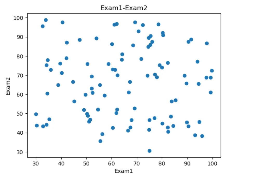
#visual the data 可视化数据
%matplotlib inline
from matplotlib import pyplot as plt
fig1 = plt.figure()
plt.scatter(data.loc[:, 'Exam1'], data.loc[:, 'Exam2'])
plt.title('Exam1-Exam2')
plt.xlabel('Exam1')
plt.ylabel('Exam2')

plt.show()
# add lable mask
mask = data.loc[:, 'Pass'] == 1
print(~mask)
0      True
1      True
2      True
3     False
4     False
      ...
95    False
96    False
97    False
98    False
99    False
Name: Pass, Length: 100, dtype: bool
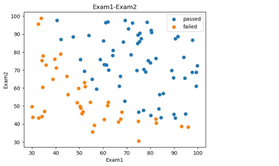
#visual the data with mask 添加标签
fig2 = plt.figure()
passed = plt.scatter(data.loc[:, 'Exam1'][mask], data.loc[:, 'Exam2'][mask])
failed = plt.scatter(data.loc[:, 'Exam1'][~mask], data.loc[:, 'Exam2'][~mask])
plt.title('Exam1-Exam2')
plt.xlabel('Exam1')
plt.ylabel('Exam2')

plt.legend((passed, failed), ('passed', 'failed'))

plt.show()
#define X,y 对变量进行数据赋值
X = data.drop(['Pass'], axis=1)
X.head()

X1 = data.loc[:, 'Exam1']
X2 = data.loc[:, 'Exam2']

X2.head()
y = data.loc[:, 'Pass']
y.head()
0    0
1    0
2    0
3    1
4    1
Name: Pass, dtype: int64
print(X.shape, y.shape)
(100, 2) (100,)
#establish the model and train it 建立并训练模型
from sklearn.linear_model import LogisticRegression
LR = LogisticRegression()
LR.fit(X,y)
LogisticRegression()
# show the pridict result and its accuracy
y_predict = LR.predict(X)
print(y_predict)
[0 0 0 1 1 0 1 0 1 1 1 0 1 1 0 1 0 0 1 1 0 1 0 0 1 1 1 1 0 0 1 1 0 0 0 0 1
 1 0 0 1 0 1 1 0 0 1 1 1 1 1 1 1 0 0 0 1 1 1 1 1 0 0 0 0 0 1 0 1 1 0 1 1 1
 1 1 1 1 0 1 1 1 1 0 1 1 0 1 1 0 1 1 0 1 1 1 1 1 0 1]
from sklearn.metrics import accuracy_score
accRet = accuracy_score(y, y_predict)

print(accRet)
0.89
#exam1 = 70 exam2 = 65
y_test = LR.predict([[75,65]])
print('passed' if y_test == 1 else 'failed')
passed


/home/changlin/anaconda3/envs/sk_env/lib/python3.7/site-packages/sklearn/base.py:451: UserWarning: X does not have valid feature names, but LogisticRegression was fitted with feature names
  "X does not have valid feature names, but"
LR.coef_
array([[0.20535491, 0.2005838 ]])
LR.intercept_
array([-25.05219314])
theta0 = LR.intercept_
theta1,theta2 = LR.coef_[0][0], LR.coef_[0][1]
print(theta0, theta1, theta2)
[-25.05219314] 0.20535491217790364 0.20058380395469022
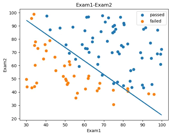
X2_new = -(theta0 + theta1 * X1)/theta2
print(X2_new)

fig3 = plt.figure()
passed = plt.scatter(data.loc[:, 'Exam1'][mask], data.loc[:, 'Exam2'][mask])
failed = plt.scatter(data.loc[:, 'Exam1'][~mask], data.loc[:, 'Exam2'][~mask])
plt.title('Exam1-Exam2')
plt.xlabel('Exam1')
plt.ylabel('Exam2')

plt.legend((passed, failed), ('passed', 'failed'))

plt.plot(X1, X2_new)
plt.show()
0     89.449169
1     93.889277
2     88.196312
3     63.282281
4     43.983773
        ...
95    39.421346
96    81.629448
97    23.219064
98    68.240049
99    48.341870
Name: Exam1, Length: 100, dtype: float64
得到一阶边界模型
下面开始建立二阶边界模型
二阶边界函数: $\mathrm{\theta_0~+\theta_1x_1~+\theta_2x_2~+\theta_3x_1^2~+\theta_4x_2^2~+\theta_5x_1x_2~=0}$
# 创建新的数据集
X1_2 = X1 * X1
X2_2 = X2 * X2
X1_X2 = X1 * X2

print(X1_2, X2_2, X1_X2)
0     1198.797805
1      917.284849
2     1285.036716
3     3621.945269
4     6246.173368
         ...
95    6970.440295
96    1786.051355
97    9863.470975
98    3062.517544
99    5591.434174
Name: Exam1, Length: 100, dtype: float64 0     6087.852690
1     1926.770807
2     5314.730478
3     7449.166166
4     5676.775061
         ...
95    2340.652054
96    7587.080849
97    4730.056948
98    4216.156574
99    8015.587398
Name: Exam2, Length: 100, dtype: float64 0     2701.500406
1     1329.435094
2     2613.354893
3     5194.273015
4     5954.672216
         ...
95    4039.229555
96    3681.156888
97    6830.430397
98    3593.334590
99    6694.671710
Length: 100, dtype: float64
X_new = {'X1':X1, 'X2':X2, 'X1_2': X1_2, 'X2_2':X2_2, 'X1_X2':X1_X2}
X_new = pd.DataFrame(X_new)
print(X_new)
           X1         X2         X1_2         X2_2        X1_X2
0   34.623660  78.024693  1198.797805  6087.852690  2701.500406
1   30.286711  43.894998   917.284849  1926.770807  1329.435094
2   35.847409  72.902198  1285.036716  5314.730478  2613.354893
3   60.182599  86.308552  3621.945269  7449.166166  5194.273015
4   79.032736  75.344376  6246.173368  5676.775061  5954.672216
..        ...        ...          ...          ...          ...
95  83.489163  48.380286  6970.440295  2340.652054  4039.229555
96  42.261701  87.103851  1786.051355  7587.080849  3681.156888
97  99.315009  68.775409  9863.470975  4730.056948  6830.430397
98  55.340018  64.931938  3062.517544  4216.156574  3593.334590
99  74.775893  89.529813  5591.434174  8015.587398  6694.671710

[100 rows x 5 columns]
# create new model and train
LR2 = LogisticRegression()
LR2.fit(X_new, y)
LogisticRegression()
# show the pridict result and its accuracy
y2_predict = LR2.predict(X_new)
print(y2_predict)
[0 0 0 1 1 0 1 1 1 1 0 0 1 1 0 1 1 0 1 1 0 1 0 0 1 1 1 0 0 0 1 1 0 1 0 0 0
 1 0 0 1 0 1 0 0 0 1 1 1 1 1 1 1 0 0 0 1 0 1 1 1 0 0 0 0 0 1 0 1 1 0 1 1 1
 1 1 1 1 0 0 1 1 1 1 1 1 0 1 1 0 1 1 0 1 1 1 1 1 1 1]
accRet2 = accuracy_score(y, y2_predict)

print(accRet2)
1.0
LR2.coef_
array([[-8.95942818e-01, -1.40029397e+00, -2.29434572e-04,
         3.93039312e-03,  3.61578676e-02]])
# 先排序 否则有交叉
X1_new = X1.sort_values()
print(X1_new)
63    30.058822
1     30.286711
57    32.577200
70    32.722833
36    33.915500
        ...
56    97.645634
47    97.771599
51    99.272527
97    99.315009
75    99.827858
Name: Exam1, Length: 100, dtype: float64
theta0 = LR2.intercept_
theta1,theta2,theta3,theta4,theta5 = LR2.coef_[0][0],LR2.coef_[0][1],LR2.coef_[0][2],LR2.coef_[0][3],LR2.coef_[0][4]

a = theta4
b = theta5 * X1_new + theta2
c = theta0 + theta1 * X1_new + theta3 * X1_new * X1_new
X2_new_bound = (-b + np.sqrt(b*b - 4*a*c))/(2*a)
# print(theta0,theta1,theta2,theta3,theta4,theta5)
print(X2_new_bound)
63    132.124249
1     130.914667
57    119.415258
70    118.725082
36    113.258684
         ...
56     39.275712
47     39.251001
51     38.963585
97     38.955634
75     38.860426
Name: Exam1, Length: 100, dtype: float64
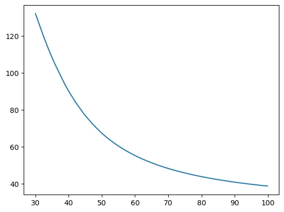
fig4 = plt.figure()
plt.plot(X1_new, X2_new_bound)
plt.show()
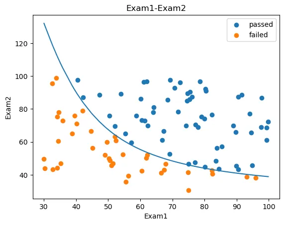
#visual the data with mask
fig5 = plt.figure()
plt.plot(X1_new, X2_new_bound)

passed = plt.scatter(data.loc[:, 'Exam1'][mask], data.loc[:, 'Exam2'][mask])
failed = plt.scatter(data.loc[:, 'Exam1'][~mask], data.loc[:, 'Exam2'][~mask])
plt.title('Exam1-Exam2')
plt.xlabel('Exam1')
plt.ylabel('Exam2')

plt.legend((passed, failed), ('passed', 'failed'))
plt.show()
二、芯片质量预测
1、基于芯片测试.csv数据,建立逻辑回归模型(二阶边界),评估模型表现
2、以函数的方式求解边界曲线
3、描绘出完整的决策边界曲线
import pandas as pd
import numpy as np
data = pd.read_csv('/root/chip_test.csv')
data.head()
<table border="1" class="dataframe"> <thead> <tr style="text-align: right;"> <th></th> <th>test1</th> <th>test2</th> <th>pass</th> </tr> </thead> <tbody> <tr> <th>0</th> <td>0.051267</td> <td>0.69956</td> <td>1</td> </tr> <tr> <th>1</th> <td>-0.092742</td> <td>0.68494</td> <td>1</td> </tr> <tr> <th>2</th> <td>-0.213710</td> <td>0.69225</td> <td>1</td> </tr> <tr> <th>3</th> <td>-0.375000</td> <td>0.50219</td> <td>1</td> </tr> <tr> <th>4</th> <td>0.183760</td> <td>0.93348</td> <td>0</td> </tr> </tbody> </table> </div>
mask = data.loc[:, 'pass'] == 1
print(~mask)
0      False
1      False
2      False
3      False
4       True
       ...
113     True
114     True
115     True
116     True
117     True
Name: pass, Length: 118, dtype: bool
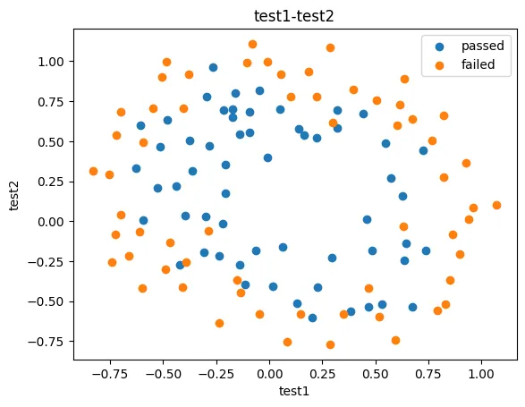
from matplotlib import pyplot as plt
fig1 = plt.figure()
passed = plt.scatter(data.loc[:, 'test1'][mask],data.loc[:, 'test2'][mask])
failed = plt.scatter(data.loc[:, 'test1'][~mask],data.loc[:, 'test2'][~mask])

plt.title("test1-test2")
plt.xlabel('test1')
plt.ylabel('test2')
plt.legend((passed,failed),('passed','failed'))
plt.show()
直接进行二阶拟合,先生成新数据
#define X,y
X = data.drop(['pass'],axis=1)
y = data.loc[:,'pass']
X1 = data.loc[:,'test1']
X2 = data.loc[:,'test2']
X1.head()
#create new data
X1_2 = X1*X1
X2_2 = X2*X2
X1_X2 = X1*X2
X_new = {'X1':X1,'X2':X2,'X1_2':X1_2,'X2_2':X2_2,'X1_X2':X1_X2}
X_new = pd.DataFrame(X_new)
print(X_new)
           X1        X2      X1_2      X2_2     X1_X2
0    0.051267  0.699560  0.002628  0.489384  0.035864
1   -0.092742  0.684940  0.008601  0.469143 -0.063523
2   -0.213710  0.692250  0.045672  0.479210 -0.147941
3   -0.375000  0.502190  0.140625  0.252195 -0.188321
4    0.183760  0.933480  0.033768  0.871385  0.171536
..        ...       ...       ...       ...       ...
113 -0.720620  0.538740  0.519293  0.290241 -0.388227
114 -0.593890  0.494880  0.352705  0.244906 -0.293904
115 -0.484450  0.999270  0.234692  0.998541 -0.484096
116 -0.006336  0.999270  0.000040  0.998541 -0.006332
117  0.632650 -0.030612  0.400246  0.000937 -0.019367

[118 rows x 5 columns]
#establish the model and train it
from sklearn.linear_model import LogisticRegression
LR2 = LogisticRegression()
LR2.fit(X_new,y)
LogisticRegression()
# 评估模型
from sklearn.metrics import accuracy_score
y2_predict = LR2.predict(X_new)
accuracy2 = accuracy_score(y,y2_predict)
print(accuracy2)
0.8135593220338984
X1_new = X1.sort_values()
theta0 = LR2.intercept_
theta1,theta2,theta3,theta4,theta5 = LR2.coef_[0][0],LR2.coef_[0][1],LR2.coef_[0][2],LR2.coef_[0][3],LR2.coef_[0][4]
a = theta4
b = theta5*X1_new+theta2
c = theta0+theta1*X1_new+theta3*X1_new*X1_new
X2_new_boundary = (-b+np.sqrt(b*b-4*a*c))/(2*a)

fig2 = plt.figure()
passed=plt.scatter(data.loc[:,'test1'][mask],data.loc[:,'test2'][mask])
failed=plt.scatter(data.loc[:,'test1'][~mask],data.loc[:,'test2'][~mask])
plt.plot(X1_new,X2_new_boundary)
plt.title('test1-test2')
plt.xlabel('test1')
plt.ylabel('test2')
plt.legend((passed,failed),('passed','failed'))
plt.show()
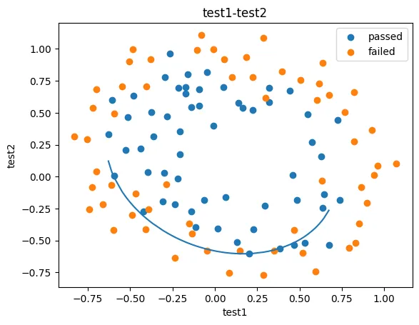
在成绩预测的例子中因为成绩不可以为负数,所以要舍去为负数的情况,这里可以为负数,不可舍去:
d = np.array(b*b-4*a*c)
d = (-b+np.sqrt(b*b-4*a*c))/(2*a)
X1_new
print(np.array(d))
[        nan         nan         nan         nan         nan         nan
         nan         nan  0.1212617   0.04679448  0.02697935  0.00872189
 -0.00830576 -0.00830576 -0.11718731 -0.16040224 -0.18016521 -0.18965258
 -0.21671004 -0.22530078 -0.23369452 -0.2499261  -0.28761583 -0.30846849
 -0.32171919 -0.32816104 -0.33448523 -0.34069505 -0.35278365 -0.35866807
 -0.37013014 -0.42186137 -0.42656594 -0.43119936 -0.43574686 -0.44021779
 -0.45318277 -0.47336128 -0.47336128 -0.48465118 -0.48828317 -0.49185073
 -0.49185073 -0.51193977 -0.51193977 -0.5181489  -0.52412149 -0.52986615
 -0.52986615 -0.53264971 -0.54066023 -0.54572074 -0.55055962 -0.55055962
 -0.55518131 -0.56170859 -0.56775529 -0.56775529 -0.58002265 -0.58002265
 -0.58588805 -0.59313744 -0.59416537 -0.59514154 -0.59852963 -0.60052615
 -0.60280757 -0.60310565 -0.60354216 -0.60379456 -0.60355793 -0.60282483
 -0.60105947 -0.60105947 -0.60047489 -0.59135016 -0.59135016 -0.59009769
 -0.5887809  -0.58285568 -0.58285568 -0.57390312 -0.56073894 -0.55572236
 -0.53219481 -0.52181028 -0.51814159 -0.51814159 -0.50647589 -0.48925514
 -0.47987024 -0.46991909 -0.45383618 -0.42349291 -0.40276684 -0.38769565
 -0.3714656  -0.353902   -0.34523055 -0.33477608 -0.33477608 -0.32451646
 -0.26416907 -0.26416907         nan         nan         nan         nan
         nan         nan         nan         nan         nan         nan
         nan         nan         nan         nan]
以函数的方式求解边界曲线:
#define f(x)

def f(x):
    a = theta4
    b = theta5*x+theta2
    c = theta0+theta1*x+theta3*x*x
    X2_new_boundary1 = (-b+np.sqrt(b*b-4*a*c))/(2*a)
    X2_new_boundary2 = (-b-np.sqrt(b*b-4*a*c))/(2*a)
    return X2_new_boundary1,X2_new_boundary2
X2_new_boundary1 = []
X2_new_boundary2 = []

for x in X1_new:
    X2_new_boundary1.append(f(x)[0])
    X2_new_boundary2.append(f(x)[1])

print(X2_new_boundary1)
[        nan         nan         nan         nan         nan         nan
         nan         nan  0.1212617   0.04679448  0.02697935  0.00872189
 -0.00830576 -0.00830576 -0.11718731 -0.16040224 -0.18016521 -0.18965258
 -0.21671004 -0.22530078 -0.23369452 -0.2499261  -0.28761583 -0.30846849
 -0.32171919 -0.32816104 -0.33448523 -0.34069505 -0.35278365 -0.35866807
 -0.37013014 -0.42186137 -0.42656594 -0.43119936 -0.43574686 -0.44021779
 -0.45318277 -0.47336128 -0.47336128 -0.48465118 -0.48828317 -0.49185073
 -0.49185073 -0.51193977 -0.51193977 -0.5181489  -0.52412149 -0.52986615
 -0.52986615 -0.53264971 -0.54066023 -0.54572074 -0.55055962 -0.55055962
 -0.55518131 -0.56170859 -0.56775529 -0.56775529 -0.58002265 -0.58002265
 -0.58588805 -0.59313744 -0.59416537 -0.59514154 -0.59852963 -0.60052615
 -0.60280757 -0.60310565 -0.60354216 -0.60379456 -0.60355793 -0.60282483
 -0.60105947 -0.60105947 -0.60047489 -0.59135016 -0.59135016 -0.59009769
 -0.5887809  -0.58285568 -0.58285568 -0.57390312 -0.56073894 -0.55572236
 -0.53219481 -0.52181028 -0.51814159 -0.51814159 -0.50647589 -0.48925514
 -0.47987024 -0.46991909 -0.45383618 -0.42349291 -0.40276684 -0.38769565
 -0.3714656  -0.353902   -0.34523055 -0.33477608 -0.33477608 -0.32451646
 -0.26416907 -0.26416907         nan         nan         nan         nan
         nan         nan         nan         nan         nan         nan
         nan         nan         nan         nan]
fig3 = plt.figure()
passed=plt.scatter(data.loc[:,'test1'][mask],data.loc[:,'test2'][mask])
failed=plt.scatter(data.loc[:,'test1'][~mask],data.loc[:,'test2'][~mask])
plt.plot(X1_new,X2_new_boundary1)
plt.plot(X1_new,X2_new_boundary2)
plt.title('test1-test2')
plt.xlabel('test1')
plt.ylabel('test2')
plt.legend((passed,failed),('passed','failed'))
plt.show()
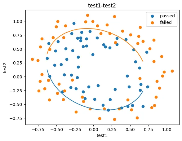
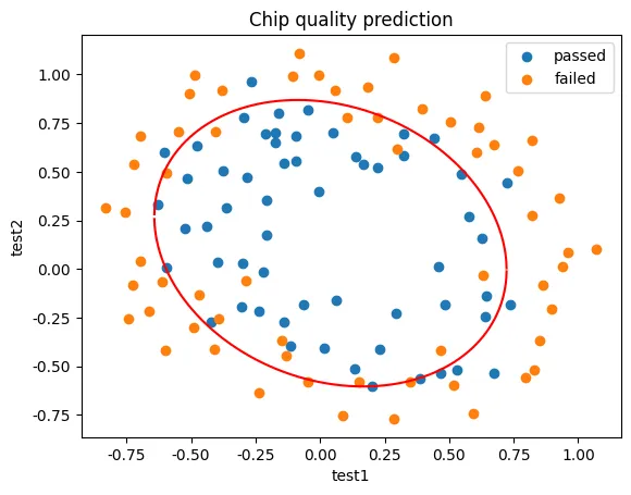
这里图的两侧缺失部分是因为test1它对应的边界上的test2的值之有间隔,所以需要生成一个新的密集X1来处理间隔问题。观察图形可发现,最小值大概是-0.9,最大值大概是1.0多一点,所以我们从-0.9开始,每个数间隔为1/10000,数是从0到19000,这样自己生成的X1就比较密集了,也就可以补全图形了。
# create x range
X1_range = [-0.9 + x/10000 for x in range(0,19000)]
X1_range = np.array(X1_range)
X2_new_boundary1 = []
X2_new_boundary2 = []
for x in X1_range:
    X2_new_boundary1.append(f(x)[0])
    X2_new_boundary2.append(f(x)[1])
# coding:utf-8
import matplotlib as mlp
fig4 = plt.figure()
passed=plt.scatter(data.loc[:,'test1'][mask],data.loc[:,'test2'][mask])
failed=plt.scatter(data.loc[:,'test1'][~mask],data.loc[:,'test2'][~mask])
plt.plot(X1_range,X2_new_boundary1,'r')
plt.plot(X1_range,X2_new_boundary2,'r')
plt.title('test1-test2')
plt.xlabel('test1')
plt.ylabel('test2')
plt.title('Chip quality prediction')
plt.legend((passed,failed),('passed','failed'))
plt.show()
这样就得到了完整的闭合二阶边界曲线: