什么是回归分析？(Regression Analysis) 回归分析是一种统计方法，用于显示两个或更多变量之间的关系。该方法检验因变量与自变量之间的关系，常用图形表示。通常情况下，自变量随因变量而变化，并且通过回归分析确定出哪些因素对该变化最重要。

回归问题

函数表达式： $$ y=f(x_1,x_2\cdots x_n) $$

其实，回归问题可以如下分类：

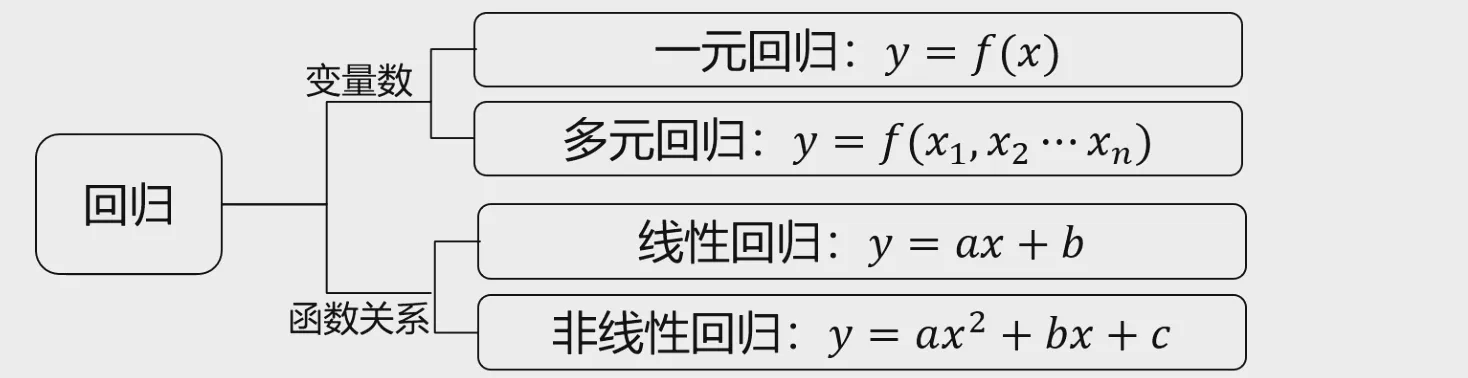
之所以称之为线性回归是因为变量与因变量之前是线性关系，比如 $$ y = ax+b $$

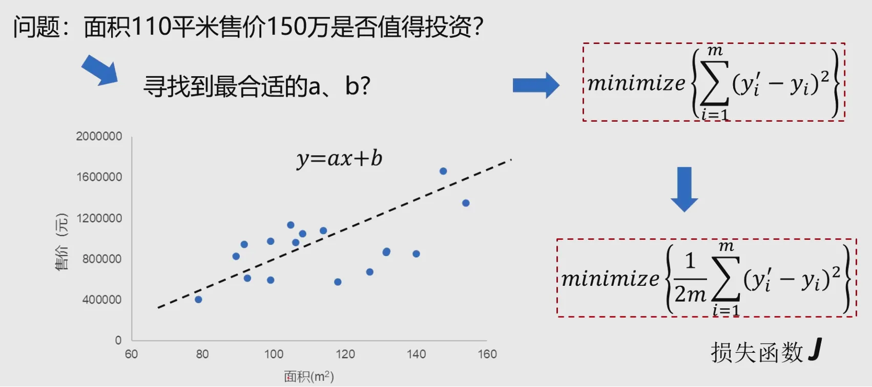
对于一组数据集，我们希望找到上面这个函数，这个函数会尽可能的拟合数据集，我们希望这个函数在X上每一个取值的函数值$X_i$与Y上每一个对应的$y_i$的平方差尽可能小。则平方损失函数如下： $$ loss(w,b)=\frac{1}{N}\sum_{i=0}^N(wx_i+b-y_i)^2 $$

梯度下降法：寻找极小值的一种方法。通过向函数上当前点对应梯度（或者是近似梯度）的反方向的规定步长距离点进行迭代搜索，直到在极小点收敛。 $$ J = f(p) $$ 具体求解方法： $$ p_{i+1}=p_i-\alpha\frac{\partial}{\partial p_i}f(p_i) $$

可以参考后面的《如何通俗理解梯度下降法》，在此不再赘述。

一元线性回归实战

基于usa_housing_price.csv数据，建立线性回归模型，预测合理房价:

1、以面积为输入变量，建立单因子模型，评估模型表现，可视化线性回归预测结果

2、以income、house age、numbers of rooms、population、area为输入变量，建立多因子模型，评估模型表现

3、预测Income=65000，House Age=5，Number of Rooms=5，Population=30000,size=200的合理房价

import pandas as pd
import numpy as np
data = pd.read_csv('usa_housing_price.csv')
data.head()
# print(type(data), data.shape)

数据如下：

<table border="1" class="dataframe"> <thead> <tr style="text-align: right;"> <th></th> <th>Avg. Area Income</th> <th>Avg. Area House Age</th> <th>Avg. Area Number of Rooms</th> <th>Area Population</th> <th>size</th> </tr> </thead> <tbody> <tr> <th>0</th> <td>79545.45857</td> <td>5.317139</td> <td>7.009188</td> <td>23086.80050</td> <td>188.214212</td> </tr> <tr> <th>1</th> <td>79248.64245</td> <td>4.997100</td> <td>6.730821</td> <td>40173.07217</td> <td>160.042526</td> </tr> <tr> <th>2</th> <td>61287.06718</td> <td>5.134110</td> <td>8.512727</td> <td>36882.15940</td> <td>227.273545</td> </tr> <tr> <th>3</th> <td>63345.24005</td> <td>3.811764</td> <td>5.586729</td> <td>34310.24283</td> <td>164.816630</td> </tr> <tr> <th>4</th> <td>59982.19723</td> <td>5.959445</td> <td>7.839388</td> <td>26354.10947</td> <td>161.966659</td> </tr> <tr> <th>...</th> <td>...</td> <td>...</td> <td>...</td> <td>...</td> <td>...</td> </tr> <tr> <th>4995</th> <td>60567.94414</td> <td>3.169638</td> <td>6.137356</td> <td>22837.36103</td> <td>161.641403</td> </tr> <tr> <th>4996</th> <td>78491.27543</td> <td>4.000865</td> <td>6.576763</td> <td>25616.11549</td> <td>159.164596</td> </tr> <tr> <th>4997</th> <td>63390.68689</td> <td>3.749409</td> <td>4.805081</td> <td>33266.14549</td> <td>139.491785</td> </tr> <tr> <th>4998</th> <td>68001.33124</td> <td>5.465612</td> <td>7.130144</td> <td>42625.62016</td> <td>184.845371</td> </tr> <tr> <th>4999</th> <td>65510.58180</td> <td>5.007695</td> <td>6.792336</td> <td>46501.28380</td> <td>148.589423</td> </tr> </tbody> </table> <p>5000 rows × 5 columns</p> </div>

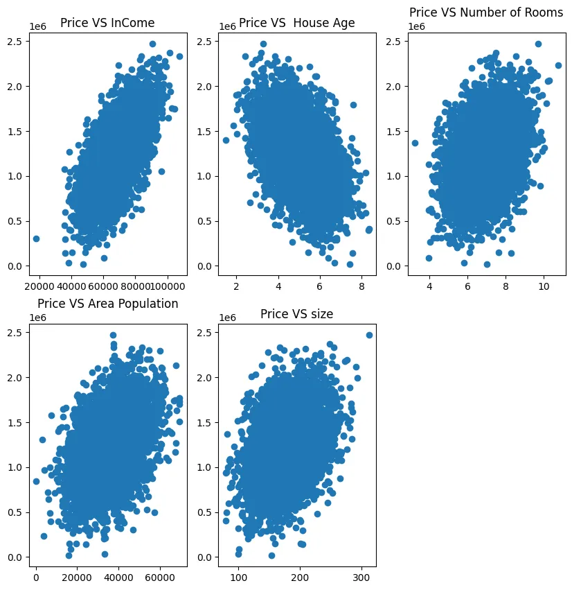
# visualize data
# 先以面积作为输入变量
from matplotlib import pyplot as plt
fig = plt.figure(figsize=(10,10))

# 子图位置限定
fig1 = plt.subplot(231)
plt.scatter(data.loc[:, 'Avg. Area Income'], data.loc[:, 'Price'])
plt.title('Price VS InCome')

fig2 = plt.subplot(232)
plt.scatter(data.loc[:, 'Avg. Area House Age'], data.loc[:, 'Price'])
plt.title('Price VS  House Age')

fig3 = plt.subplot(233)
plt.scatter(data.loc[:, 'Avg. Area Number of Rooms'], data.loc[:, 'Price'])
plt.title('Price VS Number of Rooms')

fig3 = plt.subplot(234)
plt.scatter(data.loc[:, 'Area Population'], data.loc[:, 'Price'])
plt.title('Price VS Area Population')

fig3 = plt.subplot(235)
plt.scatter(data.loc[:, 'size'], data.loc[:, 'Price'])
plt.title('Price VS size')

plt.show()

# define x and y
X = data.loc[:, 'size']
y = data.loc[:, 'Price']
# X.head()
y.head()

0    1.059034e+06
1    1.505891e+06
2    1.058988e+06
3    1.260617e+06
4    6.309435e+05
Name: Price, dtype: float64

X = np.array(X).reshape(-1,1)
print(X.shape)

(5000, 1)

# set up the linear regression model
from sklearn.linear_model import LinearRegression

LR1 = LinearRegression()

# 训练模型 train model
LR1.fit(X,y)

LinearRegression()

# 单因子预测 calc size vs price
y_predict1 = LR1.predict(X)
print(y_predict1)

[1276881.85636623 1173363.58767144 1420407.32457443 ... 1097848.86467426
 1264502.88144558 1131278.58816273]

from sklearn.metrics import mean_squared_error, r2_score

MSE_1 = mean_squared_error(y, y_predict1)
R2_1 = r2_score(y, y_predict1)
print(MSE_1, R2_1)

通过预测出来的 y_predict 的值来评估线性回归模型的表现，其中主要是通过 MSE 以及 R2_1 来作为判别的标准( MSE 的值越小越好，R2_1 的值越接近1越好)：

108771672553.62639 0.1275031240418235

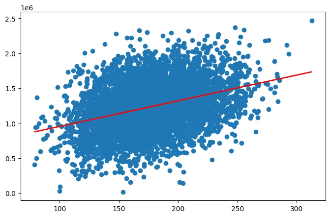
plt.figure(figsize=(8,5))
plt.scatter(X, y)
plt.plot(X,y_predict1, 'r')
plt.show()

多因子回归

以income、house age、numbers of rooms、population、area为输入变量，建立多因子模型，评估模型表现

#define X_multi
X_multi = data.drop(['Price'], axis=1)
X_multi

# setup 2nd linder model
LR_multi = LinearRegression()

#train the modle
LR_multi.fit(X_multi, y)

LinearRegression()

# make prediction 模型预测
y_predict_multi = LR_multi.predict(X_multi)
# print(y_predict_multi)

MSE_multi = mean_squared_error(y, y_predict_multi)
R2_multi = r2_score(y, y_predict_multi)

print(MSE_1, R2_1)
print(MSE_multi, R2_multi) 
# 明显可以看到比单因子回归好很多

108771672553.62639 0.1275031240418235
10219846512.17786 0.9180229195220739

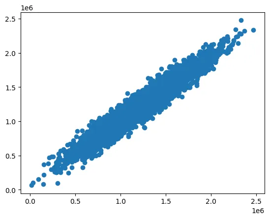
# 看看多因子回归的表现
plt.figure()
plt.scatter(y, y_predict_multi)
plt.show()

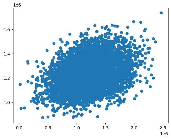
# 看看之前的单因子回归的表现
plt.figure()
plt.scatter(y, y_predict1)
plt.show()

针对具体数据进行房价预测

X_test = [65000,5,5,30000,200]
X_test = np.array(X_test).reshape(1,-1)
print(X_test, X_test.shape)

[[65000     5     5 30000   200]] (1, 5)

y_test_predict = LR_multi.predict(X_test)
print(y_test_predict)

# 完成了房价预测 [817052.19516298]

[817052.19516298]

OK，线性回归到此结束！

Reference

《如何通俗理解梯度下降法》

多因子线性回归

回归问题

一元线性回归实战

多因子回归

Reference

文章目录

评论