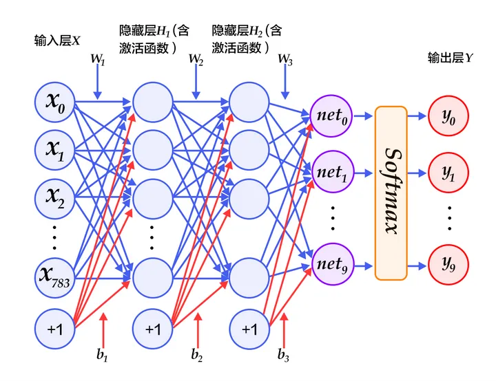
MLP实现手写数字识别
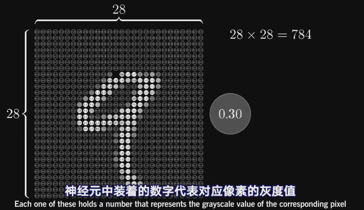
通过MLP实现手写数字识别是一个经典案例,mnist 是keras自带的一个用于手写数字识别的数据集,它的图像的分辨率是 $28 * 28$,也就是有784个像素点,它的训练集是60000个手写体图片及对应标签,测试集是10000个手写体图片及对应标签。本例中:输入层784个单元,两个隐藏层都是392个神经元,最后输出层10个单元:
关于 mnist 数据集
mnist的下载地址为: https://storage.googleapis.com/tensorflow/tf-keras-datasets/mnist.npz
mnist 的数据格式定义:
一张图片包含 $28 * 28$ 个像素,我们把这一个数组展开成一个向量,长度是 $28*28=784$。如果把数据用矩阵表示,可以把 mnist 训练数据变成一个形状为 $[60000, 7841]$ 的矩阵,第一个维度数字用来索引图片,第二个维度数字用来索引每张图片中的像素点。图片里的某个像素的强度值介于0-1之间。就像下面这样:
对于标签我们是怎么处理的呢?
mnist 数据集的标签是介于0-9的数字,我们要把标签转化为one-hot-vectors,一个one-hot向量除了某一位数字是1以外,其余维度数字都是0,比如标签0将表示为 $[1,0,0,0,0,0,0,0,0,0]$ ,标签3将表示为$[0,0,0,1,0,0,0,0,0,0]$ 。因此,可以把 mnist 训练集的标签变为 $[60000, 10]$ 的矩阵。
实战环节
首先导入数据:
from keras.datasets import mnist
(X_train,y_train),(X_test,y_test) = mnist.load_data()
print(X_train.shape, y_train.shape)
(60000, 28, 28) (60000,)
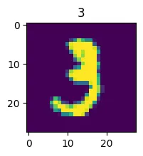
# 可视化部分数据, 看看第十个数据,是个数字3
img_1 = X_train[10]
from matplotlib import pyplot as plt
fig1 = plt.figure(figsize=(2,2))
plt.imshow(img_1)
plt.title(y_train[10])
plt.show()
feature_size = img_1.shape[0] * img_1.shape[1]
print(feature_size)

X_train_format = X_train.reshape(X_train.shape[0], feature_size)
X_test_format = X_test.reshape(X_test.shape[0], feature_size)
print(X_train_format.shape, X_test_format.shape)
784
(60000, 784) (10000, 784)
# 归一化处理
X_train_normal = X_train_format / 255
# print(X_test_format[0])
X_test_normal = X_test_format / 255
# print(X_test_format[0])
to_categorical就是将类别向量转换为二进制(只有0和1)的矩阵类型表示。其表现为将原有的类别向量转换为独热编码的形式:
#from keras.utils import to_categorical
from tensorflow.keras.utils import to_categorical
y_train_format = to_categorical(y_train)
y_test_format = to_categorical(y_test)
# 开始建立模型
from keras.models import Sequential
from keras.layers import Dense, Activation

mlp = Sequential()
mlp.add(Dense(units=392, activation='sigmoid',input_dim=feature_size))
mlp.add(Dense(units=392, activation='sigmoid'))
mlp.add(Dense(units=10, activation='softmax'))
mlp.summary()
Model: "sequential"
_________________________________________________________________
Layer (type)                 Output Shape              Param #
=================================================================
dense (Dense)                (None, 392)               307720
_________________________________________________________________
dense_1 (Dense)              (None, 392)               154056
_________________________________________________________________
dense_2 (Dense)              (None, 10)                3930
=================================================================
Total params: 465,706
Trainable params: 465,706
Non-trainable params: 0
_________________________________________________________________
关于 softmax 激活函数:在多分类问题中,我们通常会使用softmax函数作为网络输出层的激活函数,softmax函数可以对输出值进行归一化操作,把所有输出值都转化为概率,所有概率值加起来等于1,softmax的公式为:
$$ \mathrm{softmax}(x) = \frac{e^{x}}{\sum_{j} e^{x_j}} $$
# 因为不是二分类,是多分类,所以使用损失函数是categorical_crossentropy
mlp.compile(loss='categorical_crossentropy', optimizer='adam')
mlp.fit(X_train_normal, y_train_format, epochs=10)
Epoch 1/10
1875/1875 [==============================] - 6s 2ms/step - loss: 0.3441
Epoch 2/10
1875/1875 [==============================] - 4s 2ms/step - loss: 0.1459
Epoch 3/10
1875/1875 [==============================] - 4s 2ms/step - loss: 0.0940
Epoch 4/10
1875/1875 [==============================] - 4s 2ms/step - loss: 0.0651
Epoch 5/10
1875/1875 [==============================] - 5s 2ms/step - loss: 0.0479
Epoch 6/10
1875/1875 [==============================] - 5s 2ms/step - loss: 0.0357
Epoch 7/10
1875/1875 [==============================] - 4s 2ms/step - loss: 0.0260
Epoch 8/10
1875/1875 [==============================] - 5s 2ms/step - loss: 0.0215
Epoch 9/10
1875/1875 [==============================] - 5s 2ms/step - loss: 0.0157
Epoch 10/10
1875/1875 [==============================] - 4s 2ms/step - loss: 0.0146


<keras.callbacks.History at 0x19660c693a0>
# 评估一下模型
# y_train_predict = mlp.predict_classes(X_train_normal)
# print(type(y_train_predict))
from sklearn.metrics import accuracy_score
import numpy as np

y_train_predict = mlp.predict(X_train_normal)
y_train_predict = np.argmax(y_train_predict,axis=1)
print(type(y_train_predict))
print(y_train_predict[0:10])

acc_train = accuracy_score(y_train, y_train_predict)
print(acc_train)
<class 'numpy.ndarray'>
[5 0 4 1 9 2 1 3 1 4]
0.9956833333333334
# 看看测试数据集的表现
y_test_predict = mlp.predict(X_test_normal)
y_test_predict = np.argmax(y_test_predict,axis=1)
print(type(y_test_predict))
print(y_test_predict[0:10])

print(X_test_normal.shape)
acc_test = accuracy_score(y_test, y_test_predict)
print(acc_test)
<class 'numpy.ndarray'>
[7 2 1 0 4 1 4 9 5 9]
(10000, 784)
0.9791
无论是训练数据集,还是测试数据集,都还是有非常不错的表现。
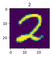
# 可视化的方式看看预测结果
img_2 = X_test[35]
fig2 = plt.figure(figsize=(2,2))
plt.imshow(img_2)
plt.title(y_test_predict[35])
plt.show()
print(X_test_normal.shape)
(10000, 784)
现在导入一张自己的图片,大小是 $28 * 28$ 的一张手写数字图片。
import cv2

fig3 = plt.figure(figsize=(2,2))
img_4 = cv2.imread('test_2.png')
plt.imshow(img_4)
plt.show()
print(img_4.shape)
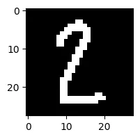
(28, 28, 3)
# 先转为灰度图
img_4_gray = cv2.cvtColor(img_4, cv2.COLOR_RGB2GRAY)
fig3 = plt.figure(figsize=(2,2))
plt.imshow(img_4_gray)
plt.show()
img_4_normal = img_4_gray / 255
newda = img_4_normal.reshape(-1, 784)

newda_predict = mlp.predict(newda)
newda_predict = np.argmax(newda_predict,axis=1)
print(type(newda_predict))
print(newda_predict)
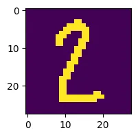
<class 'numpy.ndarray'>
[2]
可见,效果还是不错的。
需要注意的是 mnist 中的图片都是深色底图,浅色文字。所以如果拿训练好的模型去测试自己的图片需要是深色底浅色字的图才会比较准确。